



Overview
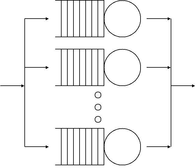
Queueing theory examines systems in which entities arrive, wait for service, and depart, using stochastic models to describe random arrival and service processes. At its core lies the queue—a line of customers, data packets, or jobs awaiting processing. By representing arrivals as a point process (often a Poisson process) and service times with probability distributions (exponential, Erlang, etc.), analysts can derive performance metrics such as the average number in system \(L\), average waiting time \(W\), and the probability of delay. These metrics guide decisions ranging from staffing a call center to sizing buffers in computer networks.A typical queueing model is denoted by Kendall’s notation A/S/c/K/N/D, where A specifies the inter‑arrival time distribution, S the service time distribution, c the number of parallel servers, K the system capacity, N the population size, and D the queue discipline (e.g., FIFO, LIFO, priority). The most celebrated example, the M/M/1 queue, assumes Markovian (memoryless) exponential inter‑arrival and service times, a single server, infinite capacity, and a first‑come‑first‑served rule. Despite its simplicity, the M/M/1 model yields closed‑form expressions such as
\[
L = \frac{\rho}{1-\rho},\qquad W = \frac{1}{\mu-\lambda},
\]
where \(\lambda\) is the arrival rate, \(\mu\) the service rate, and \(\rho = \lambda/\mu\) the traffic intensity. Extending to multiple servers (M/M/c) or non‑exponential distributions (M/G/1, G/G/1) introduces richer dynamics but retains the same conceptual framework.
Queueing theory is not limited to physical lines; it permeates telecommunications, manufacturing, health care, transportation, and computer science. In a data network, packets traverse routers that act as servers; in a hospital, patients wait for beds or physicians; in cloud computing, tasks queue for CPU cycles. By quantifying congestion and delay, queueing models enable designers to balance cost against service quality, ensuring systems operate near optimal efficiency.
History/Background
The discipline emerged in the early 20th century from the work of Agner Krarup Erlang, a Danish engineer who, in 1909, analyzed telephone call congestion for the Copenhagen Telephone Company. Erlang’s “Erlang formulas” (now known as the Erlang B and Erlang C models) provided the first analytical tools for estimating the probability of call blocking and waiting times, laying the foundation for modern telecommunications engineering.During the 1930s and 1940s, L. A. Sheppard, David G. Kendall, and William Feller expanded the theory, introducing the systematic notation (A/S/c) and exploring birth‑death processes. The post‑World‑II era saw a surge of interest as operations research (OR) matured; John D. C. Little proved his famous Little’s Law ( \(L = \lambda W\) ) in 1954, a universal relationship linking average number, arrival rate, and waiting time across all stable queueing systems.
The 1960s and 1970s brought computational advances, enabling the analysis of more complex G/G/1 and network of queues (Jackson networks). The development of Markov decision processes and queueing control theory allowed for dynamic resource allocation, such as staffing policies in service centers. In the 1990s, the rise of the Internet spurred research on packet-switched networks, leading to models like M/D/1 and fluid queues that capture bursty traffic. Today, queueing theory intersects with machine learning, stochastic optimization, and complex systems, reflecting its enduring relevance.
Key Information
- Fundamental metrics: average queue length \(L\), average waiting time \(W\), server utilization \(\rho\), probability of delay \(P_{\text{wait}}\). - Kendall’s notation (A/S/c/K/N/D) succinctly encodes model assumptions. - Little’s Law (\(L = \lambda W\)) holds for any stable, stationary queueing system, regardless of distributional specifics. - Erlang B formula (blocking probability for loss systems): \[ B(c,\rho) = \frac{\frac{\rho^{c}}{c!}}{\sum_{k=0}^{c}\frac{\rho^{k}}{k!}}. \] - Erlang C formula (probability an arriving customer must wait): \[ C(c,\rho) = \frac{\frac{\rho^{c}}{c!}\frac{c}{c-\rho}}{\sum_{k=0}^{c-1}\frac{\rho^{k}}{k!} + \frac{\rho^{c}}{c!}\frac{c}{c-\rho}}. \] - Jackson networks: collections of interconnected queues where product‑form stationary distributions enable tractable analysis of large-scale systems. - Queue disciplines: FIFO (first‑in‑first‑out), LIFO, priority, shortest‑job‑first, each influencing performance and fairness. - Applications: call‑center staffing, airport security screening, cloud‑resource provisioning, traffic signal timing, health‑care patient flow, manufacturing assembly lines.Significance
Queueing theory translates the abstract randomness of arrivals and services into concrete, actionable insights. By quantifying trade‑offs between cost (e.g., number of servers) and quality of service (e.g., waiting time), it empowers managers to make data‑driven decisions that improve customer satisfaction and operational efficiency. In telecommunications, Erlang’s formulas still underpin the design of cellular networks, ensuring call‑drop rates stay within acceptable limits. In modern cloud computing, auto‑scaling algorithms rely on queueing models to provision virtual machines just‑in‑time, reducing both latency and expense.Beyond engineering, queueing theory enriches our understanding of human behavior and societal systems. Studies of pedestrian flow, emergency evacuation, and even animal foraging patterns employ queueing concepts, revealing universal principles of congestion and resource competition. Its mathematical elegance—combining probability, Markov chains, and optimization—continues to inspire new research, especially as big data and real‑time analytics enable dynamic, adaptive queue management. In short, queueing theory is a cornerstone of systems thinking, turning the inevitable experience of waiting into a solvable, optimizable problem.